Peptide abundance profile plot

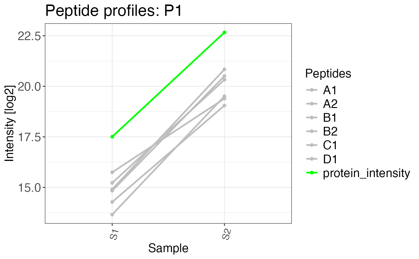
Creates a plot of peptide abundances across samples. This is helpful to investigate effects of peptide and protein abundance changes in different samples and conditions.

peptide_profile_plot(
  data,
  sample,
  peptide,
  intensity_log2,
  grouping,
  targets,
  complete_sample = FALSE,
  protein_abundance_plot = FALSE,
  interactive = FALSE,
  export = FALSE,
  export_name = "peptide_profile_plots"
)

Arguments

data

a data frame that contains at least the input variables.

sample

a character column in the data data frame that contains sample names.

peptide

a character column in the data data frame that contains peptide or precursor names.

intensity_log2

a numeric column in the data data frame that contains log2 transformed intensities.

grouping

a character column in the data data frame that contains groups by which the data should be split. This can be for example protein IDs.

targets

a character vector that specifies elements of the grouping column which should be plotted. This can also be "all" if plots for all groups should be created. Depending on the number of elements in your grouping column this can be many plots.

complete_sample

a logical value that indicates if samples that are completely missing for a given protein should be shown on the x-axis of the plot anyway. The default value is FALSE.

protein_abundance_plot

a logical value. If the input for this plot comes directly from calculate_protein_abundance this argument can be set to TRUE. This displays all peptides in gray, while the protein abundance is displayed in green.

interactive

a logical value that indicates whether the plot should be interactive (default is FALSE). If this is TRUE only one target can be supplied to the function. Interactive plots cannot be exported either.

export

a logical value that indicates if plots should be exported as PDF. The output directory will be the current working directory. The name of the file can be chosen using the export_name argument.

export_name

a character vector that provides the name of the exported file if export = TRUE.

Value

A list of peptide profile plots.

Examples

# \donttest{
# Create example data
data <- data.frame(
  sample = c(
    rep("S1", 6),
    rep("S2", 6),
    rep("S1", 2),
    rep("S2", 2)
  ),
  protein_id = c(
    rep("P1", 12),
    rep("P2", 4)
  ),
  precursor = c(
    rep(c("A1", "A2", "B1", "B2", "C1", "D1"), 2),
    rep(c("E1", "F1"), 2)
  ),
  peptide = c(
    rep(c("A", "A", "B", "B", "C", "D"), 2),
    rep(c("E", "F"), 2)
  ),
  intensity = c(
    rnorm(n = 6, mean = 15, sd = 2),
    rnorm(n = 6, mean = 21, sd = 1),
    rnorm(n = 2, mean = 15, sd = 1),
    rnorm(n = 2, mean = 15, sd = 2)
  )
)

# Calculate protein abundances and retain precursor
# abundances that can be used in a peptide profile plot
complete_abundances <- calculate_protein_abundance(
  data,
  sample = sample,
  protein_id = protein_id,
  precursor = precursor,
  peptide = peptide,
  intensity_log2 = intensity,
  method = "sum",
  for_plot = TRUE
)

# Plot protein abundance profile
# protein_abundance_plot can be set to
# FALSE to to also colour precursors
peptide_profile_plot(
  data = complete_abundances,
  sample = sample,
  peptide = precursor,
  intensity_log2 = intensity,
  grouping = protein_id,
  targets = c("P1"),
  protein_abundance_plot = TRUE
)
#> $P1

#> 
# }